Example
All examples presented bellow, as well as the example data sets used to execute them, are provided in LineStacker/Example. Methods used for plotting can be found in LineStacker/Example.
1D LineStacker
Basic usage
One dimensional example use of Line-Stacker
#This files shows basic examplpe use of
#one dimmensional stacking with LineStacker
import numpy as np
import LineStacker.OneD_Stacker
#In this example we stack 100 spectra that are located in the data folder
#and are named spectra_'+str(i) for i in range(100),
#the lines are identified with a central velocity,
#which can be found in the file 'data/central_velocity_'
#lines can be idenfified in many ways however,
#see LineStacker.OneD_Stacker.Stack for more information
numberOfSpectra=100
allImages=([0 for i in range(numberOfSpectra)])
for i in range(numberOfSpectra):
tempSpectra=np.loadtxt('data/spectra_'+str(i))
tempCenter=np.loadtxt('data/central_velocity_'+str(i))
#initializing all spectra as Image class,
#this is necessary to use OneD_Stacker.Stack
allImages[i]=LineStacker.OneD_Stacker.Image(spectrum=tempSpectra, centralVelocity=tempCenter)
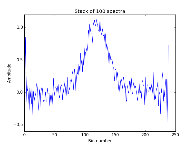
stacked=LineStacker.OneD_Stacker.Stack(allImages)
With a resulting plot looking like this:
Extended example
#This files shows a more extended examplpe use of
#one dimmensional stacking with LineStacker.
#Showcasing the bootstrapping and subsampling tools.
import numpy as np
import LineStacker.OneD_Stacker
import LineStacker.analysisTools
import LineStacker.tools.fit as fitTools
import matplotlib.pyplot as plt
#==================================================
# Stack
#==================================================
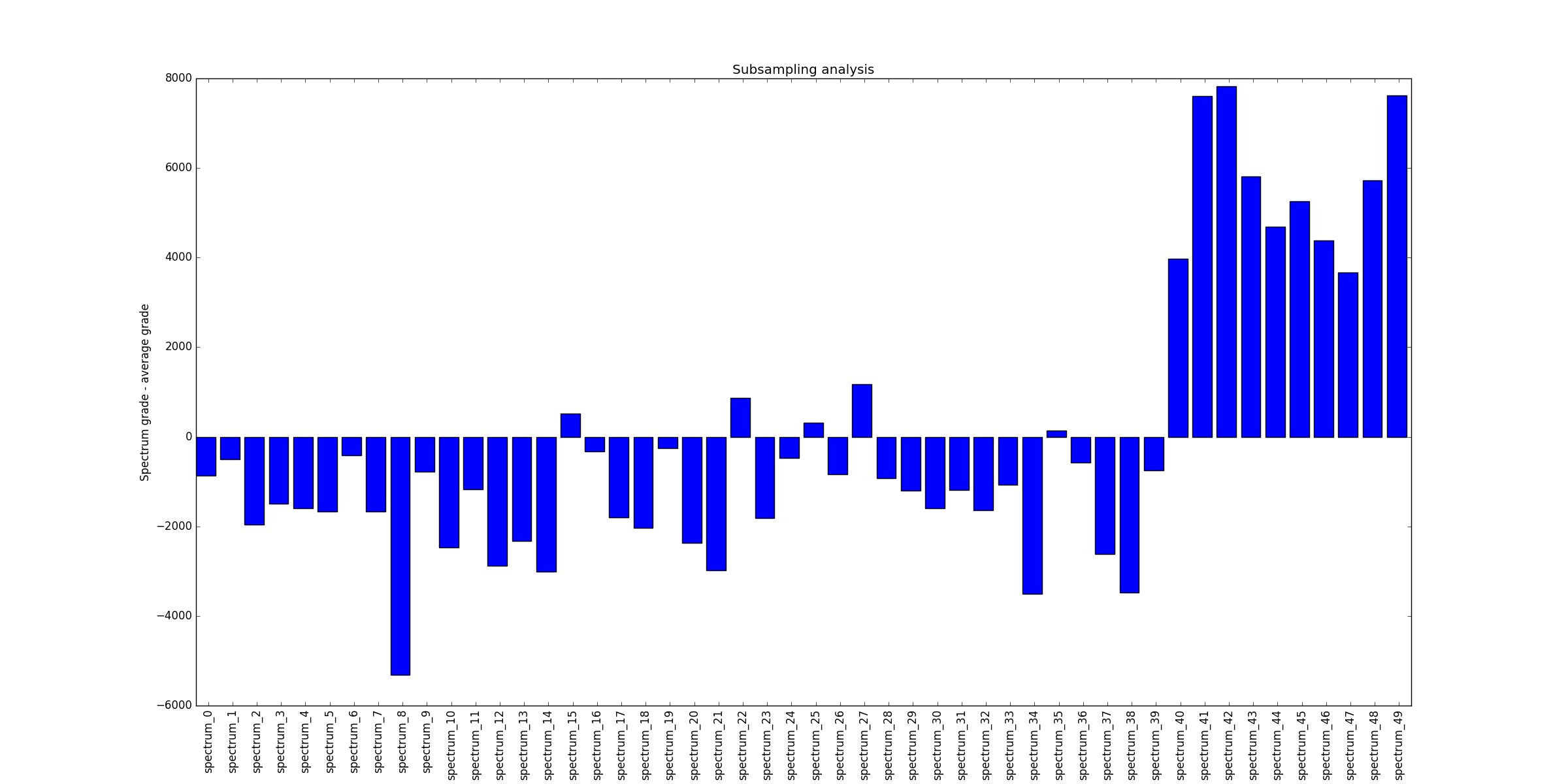
#In this example all spectra are stored in the dataExtended folder
#There are 50 spectra, 40 having a line amplitude of 1mJy (number 0 to 39)
#while 10 have a line amplitude of 10mJy (number 40 to 49).
#Spectra are simply called spectra_NUMBER with NUMBER going from 0 to 49.
#In addition to each spectra is associated
#an other file called central_velocity_NUMBER
#containing the associated central velocity.
#
#In this example we will perform a median stack of all the spectra.
#In a second time we will perform a bootstrapping analysis,
#indicating the presence of outlayers.
#Finally we will perform a subsampling analysis
#to identify these outlayers.
numberOfSpectra=50
allNames=[]
allImages=([0 for i in range(numberOfSpectra)])
#We start by initializing all spectra as LineStacker.OneD_Stacker.Image
#Which is requiered to do one dimensional stacking
for i in range(numberOfSpectra):
tempSpectra=np.loadtxt('dataExtended/spectra_'+str(i))
tempCenter=np.loadtxt('dataExtended/central_velocity_'+str(i))
allImages[i]=LineStacker.OneD_Stacker.Image( spectrum=tempSpectra,
centralVelocity=tempCenter,
name='spectrum_'+str(i))
#While the name handling is not requiered it allows easier
#treatment and understanding of the subsampling.
allNames.append(allImages[i].name)
#Here we perform the actuall stack
stacked=LineStacker.OneD_Stacker.Stack(allImages, method='median')
#The stack amplitude is stored for later vizualization
stackAmp=np.max(stacked[0])
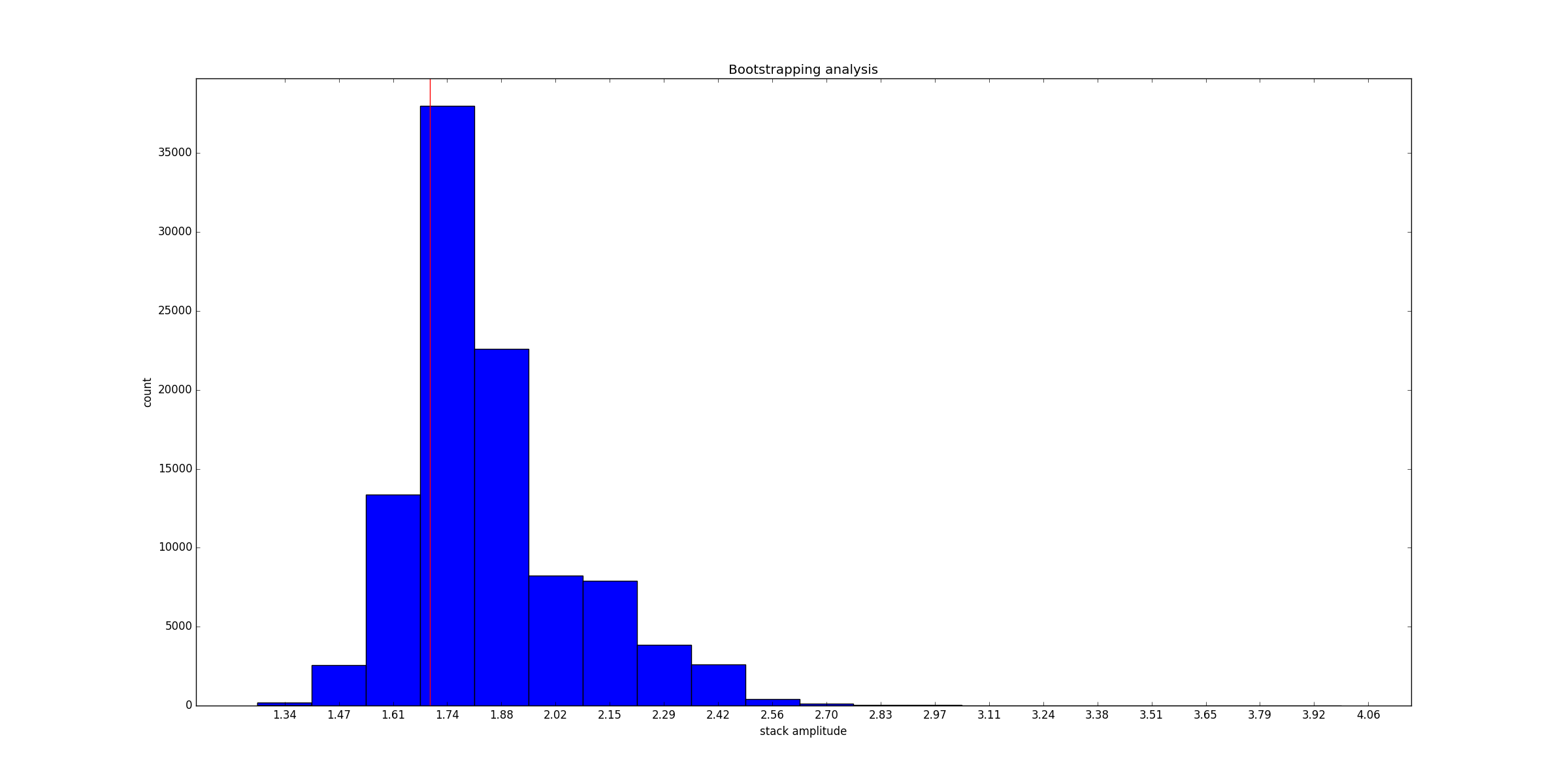
#==================================================
# bootstrapping analysis
#==================================================
bootstrapped=LineStacker.analysisTools.bootstraping_OneD( allImages,
save='amp',
nRandom=100000,
method='median')
#plotting
import matplotlib.pyplot as plt
fig=plt.figure()
ax=fig.add_subplot(111)
counts, bins, patches=ax.hist(bootstrapped, bins=20)
#for vizualization purposes...
ax.set_xticks(bins+(bins[1]-bins[0])/2)
ax.set_xticklabels(([str(bin)[:4] for bin in bins]))
#A red vertical line indicates
#the value of the amplitude of the original stack
ax.axvline(x=stackAmp, color='red')
ax.set_xlabel('stack amplitude')
ax.set_ylabel('count')
ax.set_title('Bootstrapping analysis')
fig.show()
#==================================================
#              subsampling analysis
#==================================================

subSample=LineStacker.analysisTools.subsample_OneD( allImages,
                                                    nRandom=100000,
                                                    method='median')

#plotting
fig=plt.figure()
ax=fig.add_subplot(111)
meanSub=np.mean(([subSample[i] for i in subSample]))
ax.bar(range(len(subSample)), ([subSample[name]-meanSub for name in allNames]))
ax.set_xticks(np.arange(len(allNames))+0.5)
ax.set_xticklabels(allNames, rotation='vertical')
ax.set_ylabel('Spectrum grade - average grade')
ax.set_title('Subsampling analysis')
fig.show()
Cube LineStacker
Basic usage
import LineStacker
import LineStacker.line_image
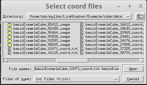
#coordinates files are selected using the GUI
coordNames=LineStacker.readCoordsNamesGUI()
coords=LineStacker.readCoords(coordNames)
#image names are identical to coordinates files,
#with '.image' replacing '_coords.txt'
imagenames=([coord.strip('_coords.txt')+'.image' for coord in coordNames])
#because redshift is used to identify the line center,
#the emission frequency is also provided
stacked=LineStacker.line_image.stack( coords,
imagenames=imagenames,
fEm=1897420620253.1646,
stampsize=16)
Here the GUI is used to select the coordinates files, it looks like this:
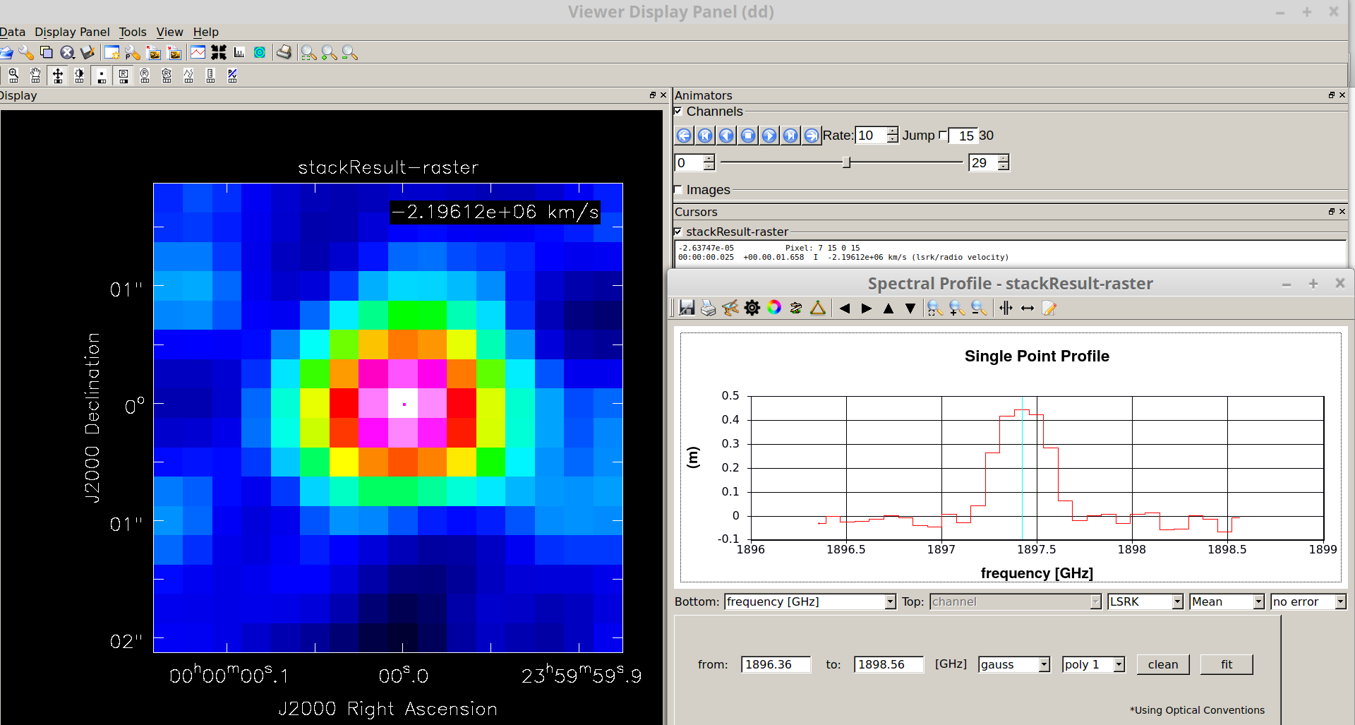
The above lines produce a stacked cube who that can be viewed with the “viewer” task in CASA:
Extended example
import LineStacker
import LineStacker.line_image
import LineStacker.analysisTools
import numpy as np
from taskinit import ia
import LineStacker.tools.fit as fitTools
import matplotlib.pyplot as plt
#coordinates files are selected using the GUI
coordNames=LineStacker.readCoordsNamesGUI()
coords=LineStacker.readCoords(coordNames)
#image names are identical to coordinates files,
#with '.image' replacing '_coords.txt'
imagenames=([coord.strip('_coords.txt')+'.image' for coord in coordNames])
#because redshift is used to identify the line center,
#the emission frequency is also provided
stacked=LineStacker.line_image.stack( coords,
imagenames=imagenames,
fEm=1897420620253.1646,
stampsize=8)
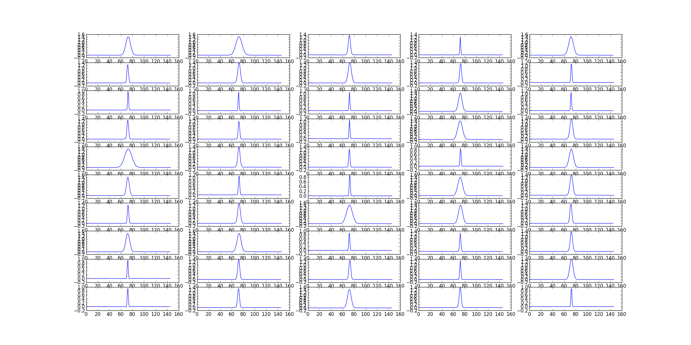
#showing every spectra
#(spectra are extracted from the central 5x5 pixels of each cube)
fig=plt.figure()
for (i,image) in enumerate(imagenames):
ia.open(image)
pix=ia.getchunk()
ia.done()
xlen=pix.shape[0]
spectrum=np.sum(pix[int(xlen/2)-2:int(xlen/2)+3,
int(xlen/2)-2:int(xlen/2)+3,
:,
:], axis=(0,1,2))
ax=fig.add_subplot(10,5,i+1)
ax.plot(spectrum)
fig.show()
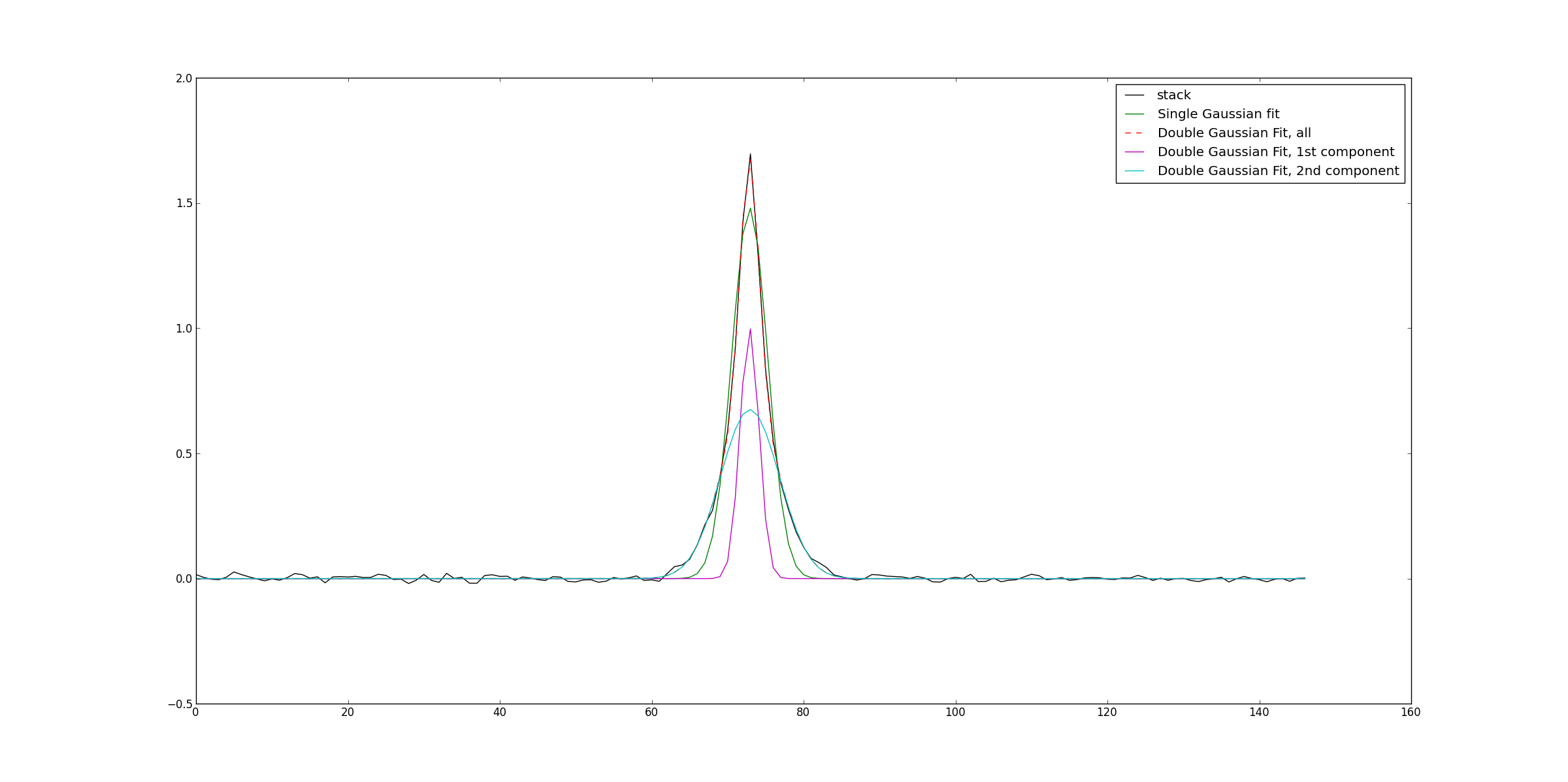
#the stack results are stored in the cube stackResult.image by default
#Here we open and extract the stacked spectra from the stacked cube,
#and fit it with 1 and 2 Gaussians
#Both the spectrum and the fits are then plotted.
ia.open('stackResult.image')
stackResultIm=ia.getchunk()
ia.done()
integratedImage=np.sum(stackResultIm, axis=(0,1,2))

fited=fitTools.GaussFit(fctToFit=integratedImage)
doubleFited=fitTools.DoubleGaussFit(fctToFit=integratedImage, returnAllComp=True)

fig=plt.figure()
ax=fig.add_subplot(111)
ax.plot(integratedImage,'k', label='stack')
ax.plot(fited, 'g', label='Single Gaussian fit')
ax.plot(doubleFited[0],'r--', label='Double Gaussian Fit, all')
ax.plot(doubleFited[1],'m', label='Double Gaussian Fit, 1st component')
ax.plot(doubleFited[2],'c', label='Double Gaussian Fit, 2nd component')
ax.legend()
fig.show()
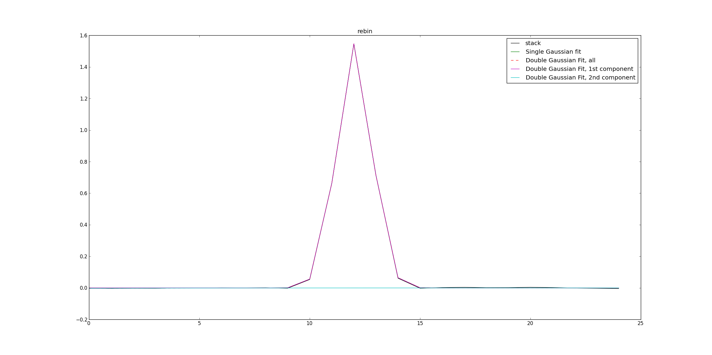
#Cubes are rebinned,
#here the linewidths used for rebenning
#are automatically identified using Gaussian fitting
rebinnedImageNames=LineStacker.analysisTools.rebin_CubesSpectra(    coords,
                                                                imagenames)

#Rebinned cubes are then stacked
rebinnedStack=LineStacker.line_image.stack(   coords,
                                                      imagenames=rebinnedImageNames,
                                                      fEm=1897420620253.1646,
                                                      stampsize=8)
#Similarly to the previous stack, spectrum is extracted, fited and plotted.
ia.open('stackResult.image')
stackResultIm=ia.getchunk()
ia.done()
integratedImage=np.sum(stackResultIm, axis=(0,1,2))

fited=fitTools.GaussFit(fctToFit=integratedImage)
doubleFited=fitTools.DoubleGaussFit(fctToFit=integratedImage, returnAllComp=True)

fig=plt.figure()
ax=fig.add_subplot(111)
ax.plot(integratedImage,'k', label='stack')
ax.plot(fited, 'g', label='Single Gaussian fit')
ax.plot(doubleFited[0],'r--', label='Double Gaussian Fit, all')
ax.plot(doubleFited[1],'m', label='Double Gaussian Fit, 1st component')
ax.plot(doubleFited[2],'c', label='Double Gaussian Fit, 2nd component')
ax.set_title('rebin')
ax.legend()
fig.show()