
LineStacker examples
All LineStacker examples in one notebook, run on the example data shipped with
LineStacker (Example/oneD and Example/cube):
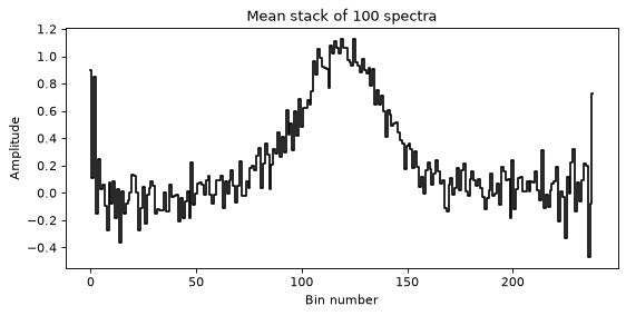
One-dimensional stacking: a basic stack of 100 spectra, then a median stack with bootstrapping and subsampling.
Cube stacking: the basic stack, with the three ways of giving the stacking positions (a catalogue, Python arrays, the coordinate files of LineStacker 1.x), then the extended example (line fits, spectral rebinning, bootstrapping).
Continuum stacking with the same function, and random-position stacks.
Run it from the Example folder. The example cubes are CASA images, so the
cube sections need CASA’s Python packages (pip install casatools);
FITS cubes would need no CASA. Everything the notebook writes goes to
notebook_outputs/.
Setup
import os
import sys
import glob

import numpy as np
import matplotlib.pyplot as plt

# Use the LineStacker of this repository (two folders up) if it is there,
# rather than another installed version.
REPO = os.path.abspath(os.path.join(os.getcwd(), '..', '..'))
if os.path.isfile(os.path.join(REPO, 'LineStacker', '__init__.py')):
    sys.path.insert(0, REPO)

import LineStacker
import LineStacker.OneD_Stacker
import LineStacker.image
import LineStacker.analysisTools
import LineStacker.tools.fit as fitTools

print('LineStacker', LineStacker.__version__, 'from', os.path.dirname(LineStacker.__file__))

EXAMPLE = os.getcwd()                         # this notebook's folder
OUT = os.path.join(EXAMPLE, 'notebook_outputs')
os.makedirs(OUT, exist_ok=True)

N_JOBS = -1                                   # Monte-Carlo tools: use all CPU cores
FEM = 1897420620253.1646                      # [CII] 158 um rest frequency (Hz)
plt.rcParams['figure.dpi'] = 80
LineStacker 2.0.1 from LineStacker
1. One-dimensional stacking
1.1 Basic stack
100 spectra (oneD/data/spectra_<i>), each with its line centre given as a
velocity (central_velocity_<i>). Every spectrum becomes a
LineStacker.OneD_Stacker.Spectrum; Stack aligns them on their line centre.
Stack returns the stacked spectrum and the number of spectra contributing to
each channel.
data = os.path.join(EXAMPLE, 'oneD', 'data')
spectra = [LineStacker.OneD_Stacker.Spectrum(spectrum=np.loadtxt(os.path.join(data, 'spectra_%d' % i)),
                                             centralVelocity=np.loadtxt(os.path.join(data, 'central_velocity_%d' % i)))
           for i in range(100)]
stacked, n_per_channel = LineStacker.OneD_Stacker.Stack(spectra)

fig, ax = plt.subplots(figsize=(8, 3.5))
ax.step(range(len(stacked)), stacked, where='mid', color='k')
ax.set_xlabel('Bin number')
ax.set_ylabel('Amplitude')
ax.set_title('Mean stack of %d spectra' % len(spectra))
plt.show()
1.2 Median stack, bootstrapping and subsampling
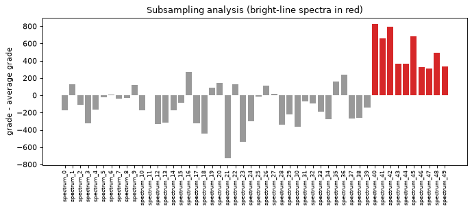
50 spectra (oneD/dataExtended): 40 have a line of amplitude 1 and 10
(numbers 40 to 49) a line of amplitude 10. Naming the spectra makes the
subsampling results readable.
data = os.path.join(EXAMPLE, 'oneD', 'dataExtended')
names = ['spectrum_%d' % i for i in range(50)]
spectra = [LineStacker.OneD_Stacker.Spectrum(spectrum=np.loadtxt(os.path.join(data, 'spectra_%d' % i)),
                                             centralVelocity=np.loadtxt(os.path.join(data, 'central_velocity_%d' % i)),
                                             name=names[i])
           for i in range(50)]
stacked, _ = LineStacker.OneD_Stacker.Stack(spectra, method='median')
stackAmp = np.max(stacked)
print('amplitude of the median stack: %.3f' % stackAmp)
amplitude of the median stack: 1.774
Bootstrapping: stack spectra drawn with replacement many times, here
saving the amplitude of each stack. The original example uses
nRandom=100000; 10 000 is enough to see the distribution and runs in seconds.
seed makes the draws reproducible, and the result does not depend on n_jobs.
bootstrapped = LineStacker.analysisTools.bootstraping_OneD(spectra, save='amp', nRandom=10000,
                                                           method='median', seed=1, n_jobs=N_JOBS)

fig, ax = plt.subplots(figsize=(8, 3.5))
ax.hist(bootstrapped, bins=30, color='0.6')
ax.axvline(stackAmp, color='red', label='stack of all spectra')
ax.set_xlabel('stack amplitude')
ax.set_ylabel('count')
ax.set_title('Bootstrapping analysis')
ax.legend()
plt.show()
LineStacker: bootstrapping 50 spectra, 10000 iterations
|          | LOADING  100%
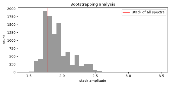
The distribution has several peaks: some draws contain more of the bright
spectra than others. Subsampling finds which spectra are responsible: random
subsets are stacked and graded (by default maximizeSNR, the signal to noise of
a Gaussian fit), and every spectrum collects the grades of the subsets it was in.
The bright spectra come out on top already with 10 000 iterations.
grades = LineStacker.analysisTools.subsample_OneD(spectra, nRandom=10000, method='median',
                                                  seed=1, n_jobs=N_JOBS)
meanGrade = np.mean(list(grades.values()))

fig, ax = plt.subplots(figsize=(10, 3.5))
ax.bar(range(len(names)), [grades[n] - meanGrade for n in names],
       color=['0.6'] * 40 + ['tab:red'] * 10)
ax.set_xticks(range(len(names)))
ax.set_xticklabels(names, rotation='vertical', fontsize=7)
ax.set_ylabel('grade - average grade')
ax.set_title('Subsampling analysis (bright-line spectra in red)')
plt.show()
LineStacker: subsampling 50 spectra, 10000 iterations
|          | LOADING  100%
2. Cube stacking
2.1 Basic stack from a catalogue
30 CASA cubes of simulated [CII] emitters (cube/data). The stacking positions
come from one table, cube/sources.csv, one row per source: its position, its
redshift and the cube it lies in (image column; relative paths are relative
to the catalogue). Positions can be in degrees or sexagesimal, with RA in hours
(CASA’s -027.40.59.866 included).
The redshift gives the line centre, so the rest frequency fEm is needed.
LineStacker prints where it wrote the stacked cube (LineStacker.verbose).
catalog = os.path.join(EXAMPLE, 'cube', 'sources.csv')
print(''.join(open(catalog).readlines()[:4]) + '...')

coords = LineStacker.readCatalog(catalog)
stacked = LineStacker.image.stack(coords, fEm=FEM, stampsize=16, N_chans=16,
                                  outfile=os.path.join(OUT, 'stackResult.fits'))   # no imagenames needed
centralValue, centralSpectrum, stackCube, missing = stacked
ra,dec,z,image
03:31:04.15,-027.40.59.866,7.26571606637,data/basicExampleCube_10071.image
03:31:15.17,-027.34.14.067,7.22190535655,data/basicExampleCube_14115.image
03:30:34.79,-027.45.34.566,7.22611675851,data/basicExampleCube_16612.image
...
LineStacker: read 30 positions in 30 cubes from sources.csv


LineStacker: mean line stack of 30 sources (16x16 pixels, 16 channels) written to LineStacker/Example/notebook_outputs/stackResult.fits
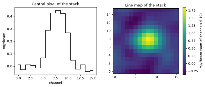
stack returns the central pixel at the central channel, the spectrum of the
central pixel, the stacked cube (axes x, y, Stokes, channel) and how many
sources miss each channel (sources whose cube does not cover it).
line = slice(6, 11)                                    # channels around the line
fig, axes = plt.subplots(1, 2, figsize=(10, 3.8))
axes[0].step(range(16), centralSpectrum * 1e3, where='mid', color='k')
axes[0].set_xlabel('channel')
axes[0].set_ylabel('mJy/beam')
axes[0].set_title('Central pixel of the stack')
im = axes[1].imshow(stackCube[:, :, 0, line].sum(axis=2).T * 1e3, origin='lower')
fig.colorbar(im, ax=axes[1], label='mJy/beam (sum of channels 6-10)')
axes[1].set_title('Line map of the stack')
plt.show()
readCatalog reads CSV, ECSV, FITS tables, VOTable (anything astropy.table
reads), an astropy Table or a pandas DataFrame. Columns can have other
names: readCatalog(cat, ra='RAJ2000', dec='DEJ2000', z='zspec', image='cube')
(common names such as RAJ2000, redshift, cube are found automatically).
An optional weight column gives weights for mean stacks. Without a z column
(or with z=None) the positions are for continuum stacking. Without an image
column, all sources must lie in the single cube given as imagenames;
LineStacker never guesses which cube a source belongs to.
2.2 The same stack from Python arrays
makeCoords builds the coordinates from lists, numpy arrays, table columns,
astropy quantities or a SkyCoord; image is one cube for all sources or one
per source. Here the arrays are the columns of the same table.
from astropy.table import Table

cat = Table.read(catalog)                                  # or your own arrays
cubes = [os.path.join(EXAMPLE, 'cube', name) for name in cat['image']]
coordsArr = LineStacker.makeCoords(cat['ra'], cat['dec'], z=cat['z'], image=cubes)

stackedArr = LineStacker.image.stack(coordsArr, fEm=FEM, stampsize=16, N_chans=16, outfile=None)
print('same stack:', np.allclose(stackedArr[2], stackCube, rtol=1e-6, atol=1e-9))
LineStacker: made 30 coordinates
LineStacker: mean line stack of 30 sources (16x16 pixels, 16 channels) done (outfile=None: not written to disk)
same stack: True
The basic forms of a position. The catalogue, the arrays and the coordinate files take positions in the same forms:
numbers in degrees (
unit='rad'for radians);sexagesimal strings with RA in hours:
03:31:04.15,03h31m04.15s, or CASA’s dotted declination-027.40.59.866;for
makeCoords, also astropy quantities or aSkyCoord;pixels of the cube, with
type='pixel'.
The frame is ICRS unless frame='fk5' (J2000) is given. Below, three sources
written four ways fall on the same pixels of their cubes.
When all the sources lie in one cube, name it once:
makeCoords(ra, dec, z=z, image='field.fits'), or leave the image out and
give imagenames='field.fits' to stack.
from astropy.coordinates import SkyCoord

first = coords[:3]                                     # three sources of the catalogue
z3, cubes3 = [c.z for c in first], [c.image for c in first]
ra_deg, dec_deg = [c.ra.deg for c in first], [c.dec.deg for c in first]

forms = {
    'degrees': LineStacker.makeCoords(ra_deg, dec_deg, z=z3, image=cubes3, verbose=False),
    'sexagesimal': LineStacker.makeCoords(['03:31:04.15', '03:31:15.17', '03:30:34.79'],        # RA in hours
                                          ['-27:40:59.866', '-27:34:14.067', '-27:45:34.566'],
                                          z=z3, image=cubes3, verbose=False),
    'SkyCoord': LineStacker.makeCoords(SkyCoord(ra_deg, dec_deg, unit='deg'), z=z3, image=cubes3, verbose=False),
}
pix = LineStacker.getPixelCoords(forms['degrees'])     # where the sources fall in their cubes
forms['pixels'] = LineStacker.makeCoords([p.x for p in pix], [p.y for p in pix], z=z3, image=cubes3,
                                         type='pixel', verbose=False)

for name, c in forms.items():
    print('%-12s' % name, '  '.join('(%.2f, %.2f)' % (p.x, p.y) for p in LineStacker.getPixelCoords(c)))
degrees      (12.07, 11.96)  (11.94, 11.96)  (12.14, 11.96)
sexagesimal  (12.07, 11.96)  (11.94, 11.96)  (12.14, 11.96)
SkyCoord     (12.07, 11.96)  (11.94, 11.96)  (12.14, 11.96)
pixels       (12.07, 11.96)  (11.94, 11.96)  (12.14, 11.96)
2.3 The same stack from coordinate files
The format of LineStacker 1.x: one coordinate file per cube
(<cube>_coord.txt, one line RA, Dec, z per source) and the list of cubes,
in the same order (LineStacker.readCoordsNamesGUI() opens a file dialog to
choose the files).
coordNames = sorted(glob.glob(os.path.join(EXAMPLE, 'cube', 'data', '*_coord.txt')))
coordsFiles = LineStacker.readCoords(coordNames)
imagenames = [c.removesuffix('_coord.txt') + '.image' for c in coordNames]

stackedFiles = LineStacker.image.stack(coordsFiles, imagenames=imagenames, fEm=FEM, stampsize=16, N_chans=16,
                                       outfile=None)
print('same stack:', np.allclose(stackedFiles[2], stackCube, rtol=1e-6, atol=1e-9))
LineStacker: read 30 positions from 30 coordinate files
LineStacker: mean line stack of 30 sources (16x16 pixels, 16 channels) done (outfile=None: not written to disk)
same stack: True
2.4 Extended example: line profiles, rebinning and bootstrapping
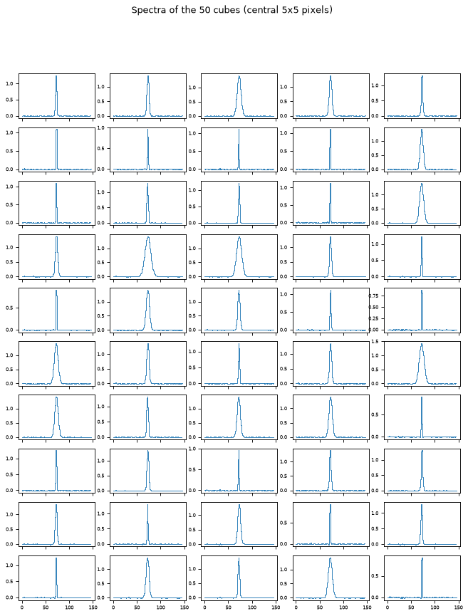
50 cubes (cube/dataExtended, catalogue cube/sources_extended.csv) whose lines have different widths. First the
stack, and the spectrum of each cube (central 5x5 pixels, read with
LineStacker.image.readCube, which reads FITS files and CASA images alike).
coords = LineStacker.readCatalog(os.path.join(EXAMPLE, 'cube', 'sources_extended.csv'))
imagenames = [c.image for c in coords]                  # one source per cube here
stacked = LineStacker.image.stack(coords, fEm=FEM, N_chans=16, stampsize=16,
                                  outfile=os.path.join(OUT, 'stackResult_extended.fits'))

fig, axes = plt.subplots(10, 5, figsize=(10, 12), sharex=True)
for ax, name in zip(axes.ravel(), imagenames):
    pix = LineStacker.image.readCube(name)
    c = pix.shape[0] // 2
    ax.step(range(pix.shape[3]), pix[c - 2:c + 3, c - 2:c + 3, :, :].sum(axis=(0, 1, 2)), where='mid', lw=0.8)
    ax.tick_params(labelsize=6)
fig.suptitle('Spectra of the 50 cubes (central 5x5 pixels)')
plt.show()
LineStacker: read 50 positions in 50 cubes from sources_extended.csv
LineStacker: mean line stack of 50 sources (16x16 pixels, 16 channels) written to LineStacker/Example/notebook_outputs/stackResult_extended.fits
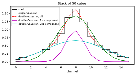
The spectrum of the stack, summed over the stamp, fitted with one and with two Gaussians. The narrow core plus broad wings come from stacking lines of different widths.
import warnings
from scipy.optimize import OptimizeWarning

def plot_fits(spectrum, x, title, xlabel):
    with warnings.catch_warnings():
        # a double Gaussian is degenerate for a single-component line
        warnings.simplefilter('ignore', OptimizeWarning)
        single = fitTools.GaussFit(fctToFit=spectrum)
        double = fitTools.DoubleGaussFit(fctToFit=spectrum, returnAllComp=True)
    fig, ax = plt.subplots(figsize=(8, 3.8))
    ax.step(x, spectrum, 'k', where='mid', label='stack')
    ax.plot(x, single, 'g', label='single Gaussian')
    ax.plot(x, double[0], 'r--', label='double Gaussian, all')
    ax.plot(x, double[1], 'm', label='double Gaussian, 1st component')
    ax.plot(x, double[2], 'c', label='double Gaussian, 2nd component')
    ax.set_xlabel(xlabel)
    ax.set_title(title)
    ax.legend(fontsize=8)
    plt.show()

integrated = stacked[2].sum(axis=(0, 1, 2))
plot_fits(integrated, range(len(integrated)), 'Stack of 50 cubes', 'channel')
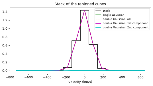
Spectral rebinning: each cube is resampled so that all lines get the width
of the narrowest one (the widths come from Gaussian fits of each cube’s
spectrum). The rebinned cubes are written to notebook_outputs/rebinned, then
stacked; the stacked line is now a single Gaussian. The velocity axis comes
from the header of the stacked cube.
A rebinned channel is the mean of the channels it covers, so all the data are
used and the line fluxes are kept. conserveFlux=False takes the value of the
spectrum at the centre of the new channel instead, as LineStacker 1.x and 2.0.0
did (see Analysis tools in the documentation).
rebinned = LineStacker.analysisTools.rebin_CubesSpectra(coords, outdir=os.path.join(OUT, 'rebinned'))
# the same positions, each in the rebinned version of its cube
newCube = dict(zip(imagenames, rebinned))
rebinnedCoords = [c.copy() for c in coords]
for c in rebinnedCoords:
    c.image = newCube[c.image]
outfile = os.path.join(OUT, 'stackResult_rebinned.fits')
rebinnedStack = LineStacker.image.stack(rebinnedCoords, fEm=FEM, N_chans=16, stampsize=16,
                                        outfile=outfile)

from astropy.io import fits
h = fits.getheader(outfile)
channels = np.arange(h['NAXIS3'])
freq = h['CRVAL3'] + (channels + 1 - h['CRPIX3']) * h['CDELT3']
velocity = 299792.458 * (h['RESTFRQ'] - freq) / h['RESTFRQ']      # radio convention, km/s
plot_fits(rebinnedStack[2].sum(axis=(0, 1, 2)), velocity, 'Stack of the rebinned cubes', 'velocity (km/s)')
LineStacker: rebinning 50 cubes to the narrowest line width
|          | LOADING  100%

LineStacker: 50 rebinned cubes written: in LineStacker/Example/notebook_outputs/rebinned (extendedExampleCube_10619_SpectralRebinned.image ... extendedExampleCube_97379_SpectralRebinned.image)
LineStacker: mean line stack of 50 sources (16x16 pixels, 16 channels) written to LineStacker/Example/notebook_outputs/stackResult_rebinned.fits
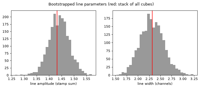
Bootstrapping the cube stack, saving the amplitude and width of a Gaussian fit of each bootstrapped stack (fits are spread over all cores).
boot = LineStacker.analysisTools.bootStraping_Cube(coords, fEm=FEM, N_chans=16,
                                                   stampsize=16, nRandom=2000, save='ampAndWidth',
                                                   seed=1, n_jobs=N_JOBS)
amp, width = np.array(boot[1:], dtype=float).T

fig, axes = plt.subplots(1, 2, figsize=(10, 3.5))
axes[0].hist(amp, bins=30, color='0.6')
axes[0].axvline(boot[0][0], color='red')
axes[0].set_xlabel('line amplitude (stamp sum)')
axes[1].hist(np.abs(width), bins=30, color='0.6')
axes[1].axvline(abs(boot[0][1]), color='red')
axes[1].set_xlabel('line width (channels)')
fig.suptitle('Bootstrapped line parameters (red: stack of all cubes)')
plt.show()
print('amplitude %.4f +- %.4f, width %.2f +- %.2f channels' % (boot[0][0], np.nanstd(amp), abs(boot[0][1]), np.nanstd(np.abs(width))))
LineStacker: bootstrapping 50 sources, 2000 iterations
|          | LOADING  100%
amplitude 1.4317 +- 0.0407, width 2.32 +- 0.26 channels
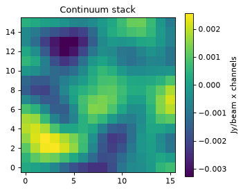
3. Continuum stacking
The same stack function: the catalogue read with z=None gives positions
without a spectral value, which are stacked as continuum (continuum=True
does the same with any positions). The example cubes have a
spectral axis, so LineStacker warns and stacks the images summed over channels
(collapse='sum', the default; 'mean' and 'median' are possible), made in
memory. Images without a spectral axis are stacked as continuum automatically,
without warning.
coords = LineStacker.readCatalog(catalog, z=None)          # continuum positions

continuum = LineStacker.image.stack(coords, stampsize=16,
                                    outfile=os.path.join(OUT, 'continuumStack.fits'))

fig, ax = plt.subplots(figsize=(4.5, 3.8))
im = ax.imshow(continuum[2][:, :, 0, 0].T, origin='lower')
fig.colorbar(im, ax=ax, label='Jy/beam x channels')
ax.set_title('Continuum stack')
plt.show()
LineStacker: read 30 positions in 30 cubes from sources.csv (z=None: continuum positions)
LineStacker: mean continuum stack of 30 sources (16x16 pixels) written to LineStacker/Example/notebook_outputs/continuumStack.fits
<cell>:3: UserWarning: continuum stacking (the coordinates have no spectral value): collapsing 30 cube(s) with a spectral axis (sum over channels) in memory
  continuum = LineStacker.image.stack(coords, stampsize=16,
Stacks at random positions tell how significant the stacked value is: each source is moved to a random position (here 4 to 9 microradians, about 0.8” to 1.9”, away; the example cubes are only 6” wide) and the stack is repeated.
random = LineStacker.analysisTools.stack_estimator(coords, continuum=True, nRandom=2000,
                                                   lowerLimit=4e-6, upperLimit=9e-6, seed=1, n_jobs=N_JOBS)
std, mean, dist = random

fig, ax = plt.subplots(figsize=(8, 3.5))
ax.hist(np.ravel(dist), bins=40, color='0.6', label='random positions')
ax.axvline(continuum[0], color='red', label='stack at the sources')
ax.set_xlabel('stacked central pixel')
ax.legend()
plt.show()
print('stack %.3g, random positions %.3g +- %.3g' % (continuum[0], mean, std))
LineStacker: stacking 2000 sets of random positions around 30 sources
|          | LOADING  100%
stack 0.00103, random positions -0.000582 +- 0.000201
<cell>:1: UserWarning: continuum stacking (continuum=True): collapsing 30 cube(s) with a spectral axis (sum over channels) in memory
  random = LineStacker.analysisTools.stack_estimator(coords, continuum=True, nRandom=2000,
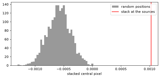
The random positions give negative values on average: they fall in the negative sidelobes of the dirty beam around each source, as the example cubes are small. On real data, use limits of several beams (the default, 5 to 10 beams).
4. Good to know
LineStacker.verbose = Falsesilences LineStacker’s messages and progress bars; any function also takesverbose=True/False.outfilenames ending in.fitsare written as FITS, other names (e.g.stackResult.image) as CASA images.The Monte-Carlo tools take
n_jobs(cores, -1 for all) andseed; results do not depend onn_jobs.